Working with Spreadsheets, by Marcus Wade

The Purpose of Working with Spreadsheets was to become more familiar with electronic spreadsheets, as they can make performing multiple calculations a much simpler process. The only tools necessary for this lab was a computer with excel software. We began initially by using excel to calculate the values of the function:

F(x)=Asin(Bx+C)

fig 1

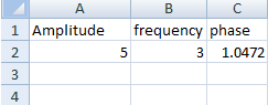
In order to achieve this, we entered in excel three straight rows of constants A (amplitude), B (frequency), and C (phase) with their respective values in the row just beneath 5, 3, and π/3 (fig 1).

fig 2

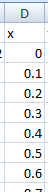
The next step was to enter all of our values for x (radians) into the column D. There were 100 values of x to calculate, from 0 to 10 in intervals of 0.1 radians. This was done quite easily by entering our first two numbers (0 and 0.1), proceeding to use the copy feature in excel to create our table of values all the way to 10 (fig 2).












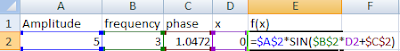
The functional values were then evaluated. The function was input entered into excel according to fig 3. The cells for constants were given ($) before and after the column header so the value remained the same, while the variable for x went through all 100 different values.

fig 3

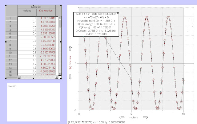
Extending the functional answers from initial x value of 0 to final x value of 10, we obtained a table of x and y values for our function. In order to see how the function behaved, the table of x and y values were copied and pasted into the graphical analysis software. The graph obtained, and the table of x and y values are shown below in fig 4. The curve fit was set to be the graph of a sin function, and the values of A, B, and C all matched the coefficients that were entered in excel originally. The only difference was the rounding off of C (π/3).

fig 4

The process was then repeated for the position function of a freely falling particle. Using the data given in the lab (-g=-9.8 m/s², v_o=50 m/s², and r_o=1000 m) we obtained our position function by integration:

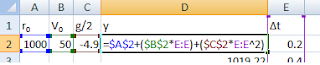
The process of entering the equation into excel was the same as for the sin function. Once again the row of constants (-g/2, v_o, and r_o) had their respective values (-4.9, 50, and 1000) placed in the rows underneath.

fig 5

The independent variable in our function is now t on the domain [0,10], with intervals of 0.2 s. Our equation was then entered into excel according to fig 5.


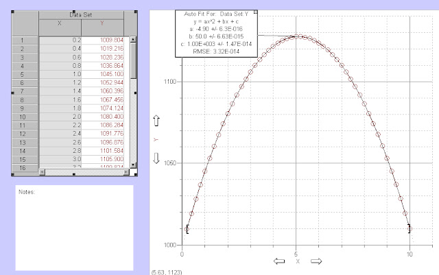
Gathering the x and y values of our function, they were once again  pasted into the graphical analysis software. A parabolic fit was applied to the graph of our data table and yielded the equation -4.9x²+50x+1000 which matched the values we obtained by integration. The graph of the freely falling particle and the table of x and y values are pictured in fig 6.

fig 6

In this lab, one learned how to use excel as a tool for entering, or gathering data and using it to do multiple calculations at once. In a lab situation in which a lot of data is taken, it would be much too tedious to work out all equations by hand. As a resulting of completing this lab, one will have extremely useful skills that will help endlessly with all other labs in the physics course.