Centripetal Force

Introduction:

The centripetal force apparatus (Pictured in Fig 1) is meant to rotate a known mass through a circular path of known radius. In timing the motion of the mass for a definite number of revolutions at roughly an equal linear speed, we can calculate the average speed. Because of the fact for uniform motion that;

Fig 1

a = V²/r

Where a = acceleration, V = velocity, and r = radius

Then;

F = (mV²)/r

Where m = mass of object

Purpose:

The purpose of the Centripetal Force lab was to verify Newton's second law of motion, specifically for the case of uniform circular motion, which is stated as follows:

F = (mV²)/r

Equipment:

Centripetal force apparatus, metric scale, vernier caliper, stop watch, slotted weight set, weight hanger, and a triple beam balance.

Setup:



fig 2

In order to obtain accurate results, the position of the mass must be such that it hangs freely over the vertical indicator when the spring is detached. Reattaching the spring, the assembly is now ready to be rotated. In order to measure the radius, the vernier caliper was used to measure the center rod to two decimal places, then dividing it by two. This result was then added to the length of the cross arm to the point where the mass was supported. This radius that was measured was 0.1754 m.


Pictured in fig 2 is the centripetal force apparatus with its respective components.








Procedure:

Beginning the experiment, the apparatus is rotated at roughly a constant speed. In order to have roughly an equal speed of rotation, the mass must be passing directly over the vertical indicator as it revolves. In timing the time (s) it takes for the apparatus to be rotated 50 revolutions across the vertical indicator, the linear average velocity can be calculated. The circumference of the circle is used in order to calculate how the far object has traveled.

C = 2πr  à   where r = radius = 0.1754m

C = 2π*0.1754 m

C = 1.1 m

Because we know that our object rotated 50 complete revolutions in the time period, then the total distance traveled is:

D = 50*C   à  Where C = 1.1 m

D = 50*1.1 m

D = 55.1 m

From the first trial run performed with the mass of 0.5 kg, the time interval that the bulb traveled 55.1 m was 38.5 s. The average linear velocity is calculated as follows:

∆r/∆t=V_avg

55.1m/ 38.5s= V_avg

V_avg = 1.43 m/s

With this data, the centripetal force can be calculated with the formula given at the beginning of the lab:

F = (mV²)/r

F_Calc = (0.5 kg *1.43 m/s^2)/0.1754 m

F_Calc = 5.84 N



fig 3

Pictured in fig 3 is the method that was taken in order to measure the amount of centripetal force. Because the spring is being stretched the same amount, the amount of force is equal. A known mass (g) was hung from a string off of the pulley in order to calculate the amount of force it takes to stretch the spring to where the bulb is directly over the vertical indicator. The mass that was measured was found to be 600 g, or 0.6 kg. The force in newtons is found as follows:

F_Meas = m*a

F_Meas = 0.6 kg * 9.8 m/s²

F_Meas = 5.88 N

Pictured below in fig 4 are the force diagrams for the forces acting both on the black bulb, as well as the mass hanging over the pulley. In both cases the net forces are zero, with no motion so all forces are balanced

fig 4

In taking the average calculated centripetal force from every trial and comparing with the result of the measurement, the amount of experimental error can be calculated. Because the average calculated centripetal force from the mass of 0.5 kg is 5.80 N, the experimental error is determined the following way:

100*((actual-calculated)/actual)

100*((5.88-5.80)/5.88)

=1.42% error

The entire process is then repeated for a new bulb mass of 0.6 kg simply by adding additional mass to the bulb.


Below in fig 5 and fig 6 are the data tables for each single trial run for bulb masses 0.5 kg as well as 0.6 kg.

fig 5

fig 6

Pictured in fig 7 and fig 8 are the percentage error data for both masses.

fig 7

fig 8

Conclusion:

Upon calculating the percentage error of the Newton's second law formula with the measured values, the results that were reached in this lab matched significantly. In the first trial run, the calculated value of centripetal force was found to be 5.84 N and the measurement was found to be 5.88 N. The difference was only 0.04 N which is arguably accurate. There were a few potential sources of error, for example:
       1) The triple beam balance used was calibrated incorrectly
       2) Although the bulb was passing over the vertical indicator, its position varied over each rotation. Certain times the bulb may have passed either few millimeters to the left or the right of the vertical indicator.
       3) The stopwatch may not have been activated or deactivated in unison with the rotation of the bulb.

Drag Force on a Coffee Filter

Introduction:

When Objects move through fluid (such as air), a drag force is exerted on the object in the direction opposing motion. It is not a constant force, as it varies with velocity. The effect and dependence of velocity on the drag force will be investigated, and the formula that we are to verify is as follows:
                                                                       F_D=k*absval(V)ⁿ 

Purpose:

The purpose of the Drag Force on a Coffee Filter lab was to learn about the relationship between drag forces and the velocity of a falling object. We were to verify that the drag force is proportional the speed of an object given by the formula:

 F_D=k*absval(V)ⁿ  

where we were to determine n's value. The accepted value of n will be 2.

Setup:

Tools used in this lab included the Logger Pro software, lab pro, motion detector, nine coffee filters, and a meter stick.

Motion Detector

The setup for this lab was relatively simple, after connecting the motion detector, turning on the computer and opening the logger pro software, the motion detector was placed on the ground facing upwards.



In this lab we were given a packet of 9 coffee filters, and it was crucial that the shape of the filters remain constant. Since the drag force depends on the formula D = (1/4)*A*v², where A = cross sectional area of the object, if the shape of our coffee changes (eg. folding), the amount of drag force being applied to our filters will become smaller. Thus, it is important that we keep our coffee filters flat.

Procedure:

The packet of 9 coffee filters had to be held at a minimum of 1.5 meters above the motion detector before it was dropped. After performing 5 trial runs for the 9 coffee filter packets, we removed one and did 5 more trial runs. this was repeated until we got down to one filter.

What should the position vs. time graph look like? It will be a quick drop in position until the terminal velocity is reached, which is when the graph becomes linear.

Fig 1

Pictured in fig 1 is the position vs. time graph of trial 4 with the linear fit of the 8 coffee filters reaching terminal velocity.

What does the slope of our line represent? It should represent the velocity that the object is traveling at once it reaches terminal velocity.











After the information for each trial run was collected,  the average speeds from each trial were taken to be the independent variable, and the number of coffee filters was taken to be our independent variable. Copying our data into the graphical analysis software, the graph pictured in fig 2 was obtained with its numeric values to the left. Once the power law fit was applied to our data plots, we obtained our experimental value for n in our equation from the beginning of the lab.

F_D=k*absval(V)ⁿ 

The equation with the fitted values was:

F_D=2.14*x^1.95 ,

Data: 

The data that was collected from each of the trial runs was put into the data table in fig 2, along with the average velocities of the 9 different coffee filter amounts.

Conclusion:

In this lab, the effect of drag forces against the velocity of our falling coffee filters was able to be determined. The more massive the object, the greater the velocity and drag force the object experiences. The errors that may have thrown off measurements in the lab include:
       1) Possible slight folding of coffee filters after release.

       2) The filters may have experienced trajectories that were not exactly perpendicular to the ground

In order to determine the amount of experimental error in this lab, the value for n that we measured was compared to the accepted value of n=2 from the drag force equation to determine the percent difference.

(100*(2-1.95))/(2)

=2.5% difference

Working with Spreadsheets, by Marcus Wade

The Purpose of Working with Spreadsheets was to become more familiar with electronic spreadsheets, as they can make performing multiple calculations a much simpler process. The only tools necessary for this lab was a computer with excel software. We began initially by using excel to calculate the values of the function:

F(x)=Asin(Bx+C)

fig 1

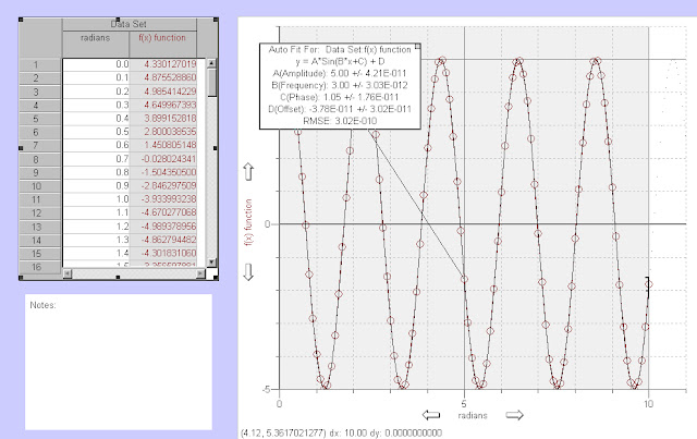
In order to achieve this, we entered in excel three straight rows of constants A (amplitude), B (frequency), and C (phase) with their respective values in the row just beneath 5, 3, and π/3 (fig 1).

fig 2

The next step was to enter all of our values for x (radians) into the column D. There were 100 values of x to calculate, from 0 to 10 in intervals of 0.1 radians. This was done quite easily by entering our first two numbers (0 and 0.1), proceeding to use the copy feature in excel to create our table of values all the way to 10 (fig 2).












The functional values were then evaluated. The function was input entered into excel according to fig 3. The cells for constants were given ($) before and after the column header so the value remained the same, while the variable for x went through all 100 different values.

fig 3

Extending the functional answers from initial x value of 0 to final x value of 10, we obtained a table of x and y values for our function. In order to see how the function behaved, the table of x and y values were copied and pasted into the graphical analysis software. The graph obtained, and the table of x and y values are shown below in fig 4. The curve fit was set to be the graph of a sin function, and the values of A, B, and C all matched the coefficients that were entered in excel originally. The only difference was the rounding off of C (π/3).

fig 4

The process was then repeated for the position function of a freely falling particle. Using the data given in the lab (-g=-9.8 m/s², v_o=50 m/s², and r_o=1000 m) we obtained our position function by integration:

The process of entering the equation into excel was the same as for the sin function. Once again the row of constants (-g/2, v_o, and r_o) had their respective values (-4.9, 50, and 1000) placed in the rows underneath.

fig 5

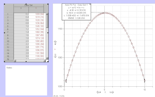
The independent variable in our function is now t on the domain [0,10], with intervals of 0.2 s. Our equation was then entered into excel according to fig 5.


Gathering the x and y values of our function, they were once again  pasted into the graphical analysis software. A parabolic fit was applied to the graph of our data table and yielded the equation -4.9x²+50x+1000 which matched the values we obtained by integration. The graph of the freely falling particle and the table of x and y values are pictured in fig 6.

fig 6

In this lab, one learned how to use excel as a tool for entering, or gathering data and using it to do multiple calculations at once. In a lab situation in which a lot of data is taken, it would be much too tedious to work out all equations by hand. As a resulting of completing this lab, one will have extremely useful skills that will help endlessly with all other labs in the physics course.